Insurance (Linear programming and discrete optimization)?
Welcome to adulthood. After three years of marriage, my friends definitely empathize, things got real and it was time to do some grown up things around our life plan. After working on Wall Street and several FinTech startups spanning personal finance, financial planning, mortgage, and property and casualty insurance…..embarrasingly I didn’t ever consider life insurance. My wife and I realized that we both should have probably gotten some earlier in our lives when things were much cheaper, but better late than never, right?
There are numerous views on how much life insurance coverage is necessary. A quick google search will populate various methods ranging from the extremely simple (i.e. a multiple X age bracket, to more complex cash flow modeling around projected income and/or expenses). For your sake, I’ll keep this post focused the fun data/math problems I solved.
Full disclaimer here again: I’m not a life insurance expert, the below was just a fun problem to explore some methods/packages I was previously unfamiliar with.
I scraped multiple policy quotes and transcribed them into a spreadsheet when I noticed something interesting. Please, see below for a glimpse into the dataframe.
| policy_id | insurer | term | coverage | yearly_premium | |
|---|---|---|---|---|---|
| 0 | 1 | Insurer 1 | 10 | $100,000 | $98.00 |
| 1 | 2 | Insurer 1 | 10 | $250,000 | $143.00 |
| 2 | 3 | Insurer 2 | 10 | $250,000 | $228.00 |
| 3 | 4 | Insurer 1 | 10 | $500,000 | $205.00 |
| 4 | 5 | Insurer 2 | 10 | $500,000 | $370.00 |
I started to wonder if this could be viewed as a potential portfolio consisting of optimal terms, coverage amounts, and, most importantly, costs. After taking a deeper look at a few plots, I started to realize how these 3 parameters have some interesting correlations, leading me to conclude that perhaps there could be a potential optimum portfolio of coverage.
plt.figure(figsize=(10, 8))
plt.scatter(x = df_matrix['term'],
            y = df_matrix['coverage'],
            s = df_matrix['yearly_premium'],
            alpha=0.3,
            edgecolors='w',)

plt.xlabel('Term')
plt.ylabel('Coverage')
plt.title('Term - Coverage - Yearly Premium', y=1.03)
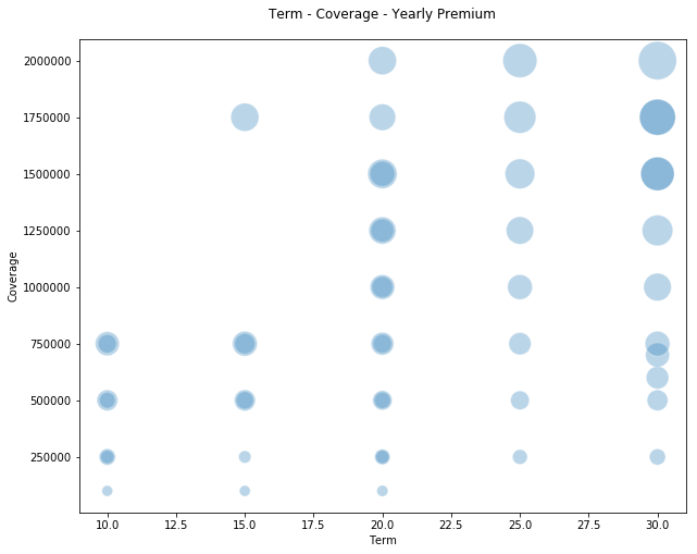
The above plot is pretty, but perhaps not very intuitive. When we try a more explicit 3-dimensional plot, it starts to get more interesting as you can visualize some real linear relationships here!
fig = plt.figure(figsize=(14, 6))
ax = fig.add_subplot(111, projection='3d')

xs = df_matrix['term']
ys = df_matrix['coverage']
zs = df_matrix['yearly_premium']
ax.scatter(xs, ys, zs, s=50, alpha=0.6, edgecolors='w')

ax.set_xlabel('Term',labelpad=10)
ax.set_ylabel('Coverage',labelpad=15)
ax.set_zlabel('Premium')

plt.show()
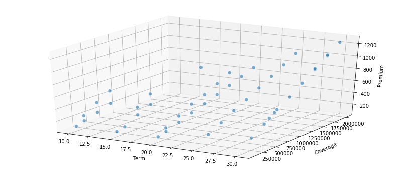
You can see the linearity is particularly pronounced along coverage amounts and premium, which is intuitive (equally important is that it is good sanity check on the data). Let’s create a new metric around premium per unit of coverage ($1,000) that helps us understand if something is “cheap” or “expensive” across all of these parameters. You can probably see where we are headed, but let’s just flush this out a bit more with some intuition before we get to the fun programming.
# Let's create a new metric
df_matrix['premium_per_thousand']=(df_matrix.yearly_premium/df_matrix.coverage)*1000
fig = plt.figure(figsize=(14, 6))
ax = fig.add_subplot(111, projection='3d')

xs = df_matrix['term']
ys = df_matrix['coverage']
zs = df_matrix['premium_per_thousand']
ax.scatter(xs, ys, zs, s=50, alpha=0.6, edgecolors='w')

ax.set_xlabel('Term',labelpad=10)
ax.set_ylabel('Coverage',labelpad=15)
ax.set_zlabel('Premium')

plt.show()
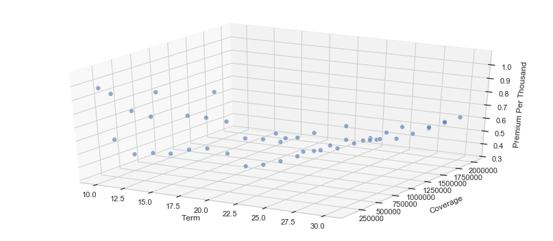
The above plot isn’t really that helpful, so let’s try another view as it seems that these relationships vary a great deal according to the term.
sns.set(style="whitegrid")
ax = sns.barplot(x=df_matrix.term.astype('str'), y=df_matrix.premium_per_thousand)
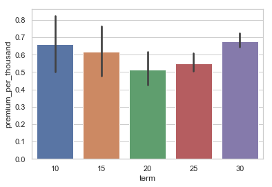
Ok, here we go, we can see here that it appears that premium per $1k of coverage is more expensive at shorter and longer terms. I speculate that shorter terms have some fixed transactional costs in them and longer terms are more expensive simply due to the fact that the longer the term the higher likelyhood of an event happening during that term period.
df_matrix.head(2)
After taking a glimpse at the dataframe below, we can clearly see the premium_per_thousand metric. If we know exactly the term we want and have a coverage amount range (and assume all insurers to be equal), we now have a metric that enables us to select the most attractively priced policy. It’s simple and elegant without a lot of complicated data science and math.
| policy_id | insurer | term | coverage | yearly_premium | monthly_premium | premium_per_thousand | |
|---|---|---|---|---|---|---|---|
| 0 | 1 | Insurer 1 | 10 | 100000.0 | 98.0 | 8.166667 | 0.980 |
| 1 | 2 | Insurer 1 | 10 | 250000.0 | 143.0 | 11.916667 | 0.572 |
Full disclaimer here again: I’m not a life insurance expert, the below was just a fun problem to explore some methods/packages I was unfamiliar with. This isn’t a recommendation on selecting life insurance.
What if we were flexible in terms of the amount of coverage we needed and the term profile? Also what if there were hypothetical instances where we can construct mult-policy portfolios with varying coverage amounts and terms over time but weighted averages that are similar to individual policies at a more attractive cost?
Hypothetical scenario: I’m interested in Policy A which has a 20 year term and for $1 million dollars of coverage our premium is $2000 per year
Policy B has a 10 year term and for $500k of coverage our premium is $300 per year Policy C has a 30 year term and for $500k of coverage our premium is $1300 per year
If I purchase policy B & C: $500k+$500k = $1 million of coverage (for the first 10 years of course then slides to $500k) ($500k10+$500k30)/($500k+$500k) = 20 years of average coverage $300+$1300 = $1600 per year
Let’s say that I really only wanted $1 million of coverage for the first 10 years, but wanted to lock in coverage over 30 years.
The above might be a fun way to explore/refresh Linear Programming/Optimization in python. Linear programming is one of the simplest ways to perform optimization (often overlooked) and is often used across many business lines. This is often used in business operations to help evaluate the trade-offs between cost and efficiency(throughput) with very complicated contraints and dependencies. I personally used this approach in optimizing call center operations where there were varying constraints on types of headcount, hours of operation, etc that really had implications on the quality of the customer experience.
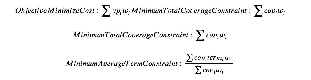
Let’s take a look at our problem, evaluating our goal or metric we’re trying to optimize which is our price (premium) here; often referred to as our objective function. The next step is to explicitly state the constraints, for example, we would need a minimum average term period of 30 years and a minimum of $1.5 million of coverage.
Next I found a python pulp package, which has some pretty good documentation.
Here we go:
df_matrix['cov_x_term']=(df_matrix.coverage * df_matrix.term)
# Create a list of the insurance items, terms, coverage, premiums, etc.
insurance_items = list(df_matrix['policy_id'])
term = dict(zip(insurance_items,df_matrix['term']))
coverage = dict(zip(insurance_items,df_matrix['coverage']))
yearly_premium = dict(zip(insurance_items,df_matrix['yearly_premium']))
cov_x_term = dict(zip(insurance_items,df_matrix['cov_x_term']))
df_matrix.head(15)
| policy_id | insurer | term | coverage | yearly_premium | monthly_premium | premium_per_thousand | cov_x_term | |
|---|---|---|---|---|---|---|---|---|
| 0 | 1 | Insurer 1 | 10 | 100000.0 | 98.0 | 8.166667 | 0.980000 | 1000000.0 |
| 1 | 2 | Insurer 1 | 10 | 250000.0 | 143.0 | 11.916667 | 0.572000 | 2500000.0 |
| 2 | 3 | Insurer 2 | 10 | 250000.0 | 228.0 | 19.000000 | 0.912000 | 2500000.0 |
| 3 | 4 | Insurer 1 | 10 | 500000.0 | 205.0 | 17.083333 | 0.410000 | 5000000.0 |
| 4 | 5 | Insurer 2 | 10 | 500000.0 | 370.0 | 30.833333 | 0.740000 | 5000000.0 |
| 5 | 6 | Insurer 1 | 10 | 750000.0 | 277.0 | 23.083333 | 0.369333 | 7500000.0 |
| 6 | 7 | Insurer 3 | 10 | 750000.0 | 488.0 | 40.666667 | 0.650667 | 7500000.0 |
| 7 | 8 | Insurer 1 | 15 | 100000.0 | 100.0 | 8.333333 | 1.000000 | 1500000.0 |
| 8 | 9 | Insurer 1 | 15 | 250000.0 | 130.0 | 10.833333 | 0.520000 | 3750000.0 |
| 9 | 10 | Insurer 1 | 15 | 500000.0 | 250.0 | 20.833333 | 0.500000 | 7500000.0 |
| 10 | 11 | Insurer 3 | 15 | 500000.0 | 378.0 | 31.500000 | 0.756000 | 7500000.0 |
| 11 | 12 | Insurer 1 | 15 | 750000.0 | 345.0 | 28.750000 | 0.460000 | 11250000.0 |
| 12 | 13 | Insurer 3 | 15 | 750000.0 | 521.0 | 43.416667 | 0.694667 | 11250000.0 |
| 13 | 14 | Insurer 1 | 15 | 1750000.0 | 666.0 | 55.500000 | 0.380571 | 26250000.0 |
| 14 | 15 | Insurer 1 | 20 | 100000.0 | 105.0 | 8.750000 | 1.050000 | 2000000.0 |
Now let’s setup a framework to solve this thing with linear programming. In this case it’ll be integer programming as we can’t have fractional weights, i.e. .3 of an insurance policy, we can only have integers.
from pulp import *
min_avg_term = 30
min_tot_cov = 1500000
prob = LpProblem("Insurance Problem",LpMinimize)
insurance_vars = LpVariable.dicts("Life",insurance_items,0,cat='Integer')
#Objective is the lowest yearly premium
prob += lpSum([yearly_premium[i]*insurance_vars[i] for i in insurance_items])

#Minimum Total Coverage
prob += lpSum([coverage[f] * insurance_vars[f] for f in insurance_items]) >= min_tot_cov, "MinimumTotalCoverage"

#Minimum Average Term
prob += lpSum([cov_x_term[f] * insurance_vars[f] for f in insurance_items]) >= min_avg_term*(lpSum([coverage[f] * insurance_vars[f] for f in insurance_items])), "MinimumAvgDuration"

prob.solve()

print("Status:", LpStatus[prob.status])
Status: Optimal
#Now we have a dictionary that has a series of variables and an optimal set of weights for example
print (prob.variables()[3].varValue)
```    0.0


```python
#Let's grab all the weights and put them into a dataframe so we can easily take a look
weights_dict = {}
pricing_dict = {}

weights_dict={}
for v in prob.variables():
    weights_dict.update({v.name[5:]:v.varValue})
weights_df = pd.DataFrame(weights_dict,index=[0]).transpose()
weights_df.reset_index(inplace=True)
weights_df.rename(columns={'index':'policy_id',0:'weights'},inplace=True)
#formatting these fields so we can compare them to the original matrix
weights_df.policy_id = weights_df.policy_id.apply(lambda l: float(l))
weights_df.weights = weights_df.weights.apply(lambda l: float(l))
weights_df.info()
<class 'pandas.core.frame.DataFrame'>
RangeIndex: 49 entries, 0 to 48
Data columns (total 2 columns):
policy_id    49 non-null float64
weights      49 non-null float64
dtypes: float64(2)
memory usage: 864.0 bytes
weights_df[weights_df.weights>0.0]
| policy_id | weights | |
|---|---|---|
| 39 | 45.0 | 1.0 |
There is only 1 policy that has a weight equal to 1 for a minimum average term of 30 years and $1.5 million of coverage. It appears that for these constraints, this policy is optimally priced.
df_scenario = df_matrix.merge(weights_df,how='left',on='policy_id')
df_scenario.tail()
| policy_id | insurer | term | coverage | yearly_premium | monthly_premium | premium_per_thousand | cov_x_term | weights | |
|---|---|---|---|---|---|---|---|---|---|
| 44 | 45 | Insurer 1 | 30 | 1500000.0 | 941.0 | 78.416667 | 0.627333 | 45000000.0 | 1.0 |
| 45 | 46 | Insurer 2 | 30 | 1500000.0 | 955.0 | 79.583333 | 0.636667 | 45000000.0 | 0.0 |
| 46 | 47 | Insurer 1 | 30 | 1750000.0 | 1087.0 | 90.583333 | 0.621143 | 52500000.0 | 0.0 |
| 47 | 48 | Insurer 2 | 30 | 1750000.0 | 1100.0 | 91.666667 | 0.628571 | 52500000.0 | 0.0 |
| 48 | 49 | Insurer 2 | 30 | 2000000.0 | 1234.0 | 102.833333 | 0.617000 | 60000000.0 | 0.0 |
df_scenario[df_scenario.weights>0.0]
| policy_id | insurer | term | coverage | yearly_premium | monthly_premium | premium_per_thousand | cov_x_term | weights | |
|---|---|---|---|---|---|---|---|---|---|
| 44 | 45 | Insurer 1 | 30 | 1500000.0 | 941.0 | 78.416667 | 0.627333 | 45000000.0 | 1.0 |
Perhaps, let’s look at a few different scenarios of coverage and term. It is expected that the common policy terms 10, 20, and 30 years are likely optimally priced. So, perhaps looking at some potential terms in the middle may yield some fruit from using our integer programming technique/tool.
# coverage
min_cov_array = [750000,1000000,1250000,1500000,1750000,2000000]
min_term_array = [15,20,23,25,27]
num_scenarios = len(min_cov_array)*len(min_term_array)

weights_dict = {}
pricing_dict = {}

df_scenario = pd.DataFrame()
df_final_scenario_policy_weights = pd.DataFrame()
df_final_summary = pd.DataFrame()

#min_avg_term = 25.0
for min_avg_term in min_term_array:
    #Can break below into sub_function
    for min_tot_cov in min_cov_array:
        #keep data on each run remember scenario for min_avg_term

        prob = LpProblem("Insurance Problem",LpMinimize)
        insurance_vars = LpVariable.dicts("Life",insurance_items,0,cat='Integer')

        prob += lpSum([yearly_premium[i]*insurance_vars[i] for i in insurance_items])
        prob += lpSum([coverage[f] * insurance_vars[f] for f in insurance_items]) >= min_tot_cov, "MinimumTotalCoverage"
        prob += lpSum([cov_x_term[f] * insurance_vars[f] for f in insurance_items]) >= min_avg_term*(lpSum([coverage[f] * insurance_vars[f] for f in insurance_items])), "MinimumAvgDuration"
        prob.solve()

        weights_dict[f'{min_avg_term}_{min_tot_cov:}']={}
        for v in prob.variables():
            weights_dict[f'{min_avg_term}_{min_tot_cov:}'].update({v.name[5:]:v.varValue})

    #write all this into dataframe
    weights_df = pd.DataFrame(weights_dict)
    weights_df.reset_index(inplace=True)
    weights_df.rename(columns={'index':'policy_id'},inplace=True)

    weights_df['policy_id'] = weights_df['policy_id'].astype('int64')

    df_scenario = df_matrix.merge(weights_df,how='left',on='policy_id')
num_scenarios: 30
30
weights_df.shape
(49, 31)
df_scenario.head(5)
| policy_id | insurer | term | coverage | yearly_premium | monthly_premium | premium_per_thousand | cov_x_term | 15_750000 | 15_1000000 | ... | 25_1250000 | 25_1500000 | 25_1750000 | 25_2000000 | 27_750000 | 27_1000000 | 27_1250000 | 27_1500000 | 27_1750000 | 27_2000000 | |
|---|---|---|---|---|---|---|---|---|---|---|---|---|---|---|---|---|---|---|---|---|---|
| 0 | 1 | Insurer 1 | 10 | 100000.0 | 98.0 | 8.166667 | 0.980 | 1000000.0 | 0.0 | 0.0 | ... | 0.0 | 0.0 | 0.0 | 0.0 | 0.0 | 0.0 | 0.0 | 0.0 | 0.0 | 0.0 |
| 1 | 2 | Insurer 1 | 10 | 250000.0 | 143.0 | 11.916667 | 0.572 | 2500000.0 | 0.0 | 0.0 | ... | 0.0 | 0.0 | 0.0 | 0.0 | 0.0 | 0.0 | 0.0 | 0.0 | 0.0 | 0.0 |
| 2 | 3 | Insurer 2 | 10 | 250000.0 | 228.0 | 19.000000 | 0.912 | 2500000.0 | 0.0 | 0.0 | ... | 0.0 | 0.0 | 0.0 | 0.0 | 0.0 | 0.0 | 0.0 | 0.0 | 0.0 | 0.0 |
| 3 | 4 | Insurer 1 | 10 | 500000.0 | 205.0 | 17.083333 | 0.410 | 5000000.0 | 0.0 | 0.0 | ... | 0.0 | 0.0 | 0.0 | 0.0 | 0.0 | 0.0 | 0.0 | 0.0 | 0.0 | 0.0 |
| 4 | 5 | Insurer 2 | 10 | 500000.0 | 370.0 | 30.833333 | 0.740 | 5000000.0 | 0.0 | 0.0 | ... | 0.0 | 0.0 | 0.0 | 0.0 | 0.0 | 0.0 | 0.0 | 0.0 | 0.0 | 0.0 |
5 rows × 38 columns
# for a more convenient view let's only keep the policies that have weights > 0
df_scenario.shape
(49, 38)
## for illustrative purposes I'm copying this over to a separate dataframe, with large datasets this is not recommended.
df_weighted = df_scenario[(df_scenario.iloc[:,-num_scenarios:]!=0).any(axis=1)]
df_weighted = df_weighted.copy()
df_weighted.shape
(19, 38)
# can see your composition of policies for each optimized scenario
df_weighted.head(5)
| policy_id | insurer | term | coverage | yearly_premium | monthly_premium | premium_per_thousand | cov_x_term | 15_750000 | 15_1000000 | ... | 25_1250000 | 25_1500000 | 25_1750000 | 25_2000000 | 27_750000 | 27_1000000 | 27_1250000 | 27_1500000 | 27_1750000 | 27_2000000 | |
|---|---|---|---|---|---|---|---|---|---|---|---|---|---|---|---|---|---|---|---|---|---|
| 8 | 9 | Insurer 1 | 15 | 250000.0 | 130.0 | 10.833333 | 0.520000 | 3750000.0 | 0.0 | 0.0 | ... | 0.0 | 0.0 | 0.0 | 0.0 | 0.0 | 0.0 | 1.0 | 1.0 | 0.0 | 0.0 |
| 17 | 18 | Insurer 1 | 20 | 500000.0 | 215.0 | 17.916667 | 0.430000 | 10000000.0 | 0.0 | 0.0 | ... | 0.0 | 0.0 | 0.0 | 0.0 | 0.0 | 0.0 | 0.0 | 0.0 | 1.0 | 1.0 |
| 19 | 20 | Insurer 1 | 20 | 750000.0 | 292.0 | 24.333333 | 0.389333 | 15000000.0 | 1.0 | 0.0 | ... | 0.0 | 0.0 | 0.0 | 0.0 | 0.0 | 0.0 | 0.0 | 0.0 | 0.0 | 0.0 |
| 21 | 22 | Insurer 1 | 20 | 1000000.0 | 365.0 | 30.416667 | 0.365000 | 20000000.0 | 0.0 | 1.0 | ... | 0.0 | 0.0 | 0.0 | 0.0 | 0.0 | 0.0 | 0.0 | 0.0 | 0.0 | 0.0 |
| 23 | 24 | Insurer 1 | 20 | 1250000.0 | 442.0 | 36.833333 | 0.353600 | 25000000.0 | 0.0 | 0.0 | ... | 0.0 | 0.0 | 0.0 | 0.0 | 0.0 | 0.0 | 0.0 | 0.0 | 0.0 | 0.0 |
5 rows × 38 columns
Below, I have listed a few scenarios with policies > 1, which indicates that a combination of policies will yield a more optimal price!
#Quick view of our policies shows that this may be working.
df_weighted.iloc[:,-num_scenarios:].astype(bool).sum()
15_750000     1
15_1000000    1
15_1250000    1
15_1500000    1
15_1750000    1
15_2000000    1
20_750000     1
20_1000000    1
20_1250000    1
20_1500000    1
20_1750000    1
20_2000000    1
23_750000     1
23_1000000    1
23_1250000    2
23_1500000    2
23_1750000    2
23_2000000    2
25_750000     1
25_1000000    1
25_1250000    1
25_1500000    1
25_1750000    1
25_2000000    1
27_750000     1
27_1000000    1
27_1250000    2
27_1500000    2
27_1750000    2
27_2000000    2
dtype: int64
aggregate = {}
for i in df_weighted.iloc[:,-num_scenarios:].columns:
    aggregate[i]={
                'policy_count':df_weighted[i].astype(bool).sum(),
                'yearly_premium':np.dot(df_weighted.yearly_premium,df_weighted[i]),
                'wa_term':np.dot(df_weighted['cov_x_term'],df_weighted[i])/(np.dot(df_weighted.coverage,df_weighted[i])),
                'total_coverage':np.dot(df_weighted.coverage,df_weighted[i])}
#count number of unique policies
df_portfolio_stats = pd.DataFrame(aggregate).transpose()
df_portfolio_stats.index.rename('scenario',inplace=True)
df_portfolio_stats.reset_index(inplace=True)
df_portfolio_stats['min_avg_term']=df_portfolio_stats.scenario.str.split("_",expand=True)[0]
df_portfolio_stats['min_tot_cov']=df_portfolio_stats.scenario.str.split("_",expand=True)[1]
df_portfolio_stats = df_portfolio_stats[['scenario', 'min_avg_term','min_tot_cov','policy_count', 'yearly_premium', 'wa_term','total_coverage']]
df_portfolio_stats['premium_per_thousand']=(df_portfolio_stats.yearly_premium/df_portfolio_stats.total_coverage)*1000
Now we have everything in a format that allows us to compare to our original price matrix; personally I was intrigued by 23_1500000,23_1750000,23_2000000.
Enjoy!
df_portfolio_stats.head(10)
| scenario | min_avg_term | min_tot_cov | policy_count | yearly_premium | wa_term | total_coverage | premium_per_thousand | |
|---|---|---|---|---|---|---|---|---|
| 0 | 15_750000 | 15 | 750000 | 1.0 | 292.0 | 20.000000 | 750000.0 | 0.389333 |
| 1 | 15_1000000 | 15 | 1000000 | 1.0 | 365.0 | 20.000000 | 1000000.0 | 0.365000 |
| 2 | 15_1250000 | 15 | 1250000 | 1.0 | 442.0 | 20.000000 | 1250000.0 | 0.353600 |
| 3 | 15_1500000 | 15 | 1500000 | 1.0 | 518.0 | 20.000000 | 1500000.0 | 0.345333 |
| 4 | 15_1750000 | 15 | 1750000 | 1.0 | 594.0 | 20.000000 | 1750000.0 | 0.339429 |
| 5 | 15_2000000 | 15 | 2000000 | 1.0 | 671.0 | 20.000000 | 2000000.0 | 0.335500 |
| 6 | 20_750000 | 20 | 750000 | 1.0 | 292.0 | 20.000000 | 750000.0 | 0.389333 |
| 7 | 20_1000000 | 20 | 1000000 | 1.0 | 365.0 | 20.000000 | 1000000.0 | 0.365000 |
| 8 | 20_1250000 | 20 | 1250000 | 1.0 | 442.0 | 20.000000 | 1250000.0 | 0.353600 |
| 9 | 20_1500000 | 20 | 1500000 | 1.0 | 518.0 | 20.000000 | 1500000.0 | 0.345333 |
| 10 | 20_1750000 | 20 | 1750000 | 1.0 | 594.0 | 20.000000 | 1750000.0 | 0.339429 |
| 11 | 20_2000000 | 20 | 2000000 | 1.0 | 671.0 | 20.000000 | 2000000.0 | 0.335500 |
| 12 | 23_750000 | 23 | 750000 | 1.0 | 417.0 | 25.000000 | 750000.0 | 0.556000 |
| 13 | 23_1000000 | 23 | 1000000 | 1.0 | 520.0 | 25.000000 | 1000000.0 | 0.520000 |
| 14 | 23_1250000 | 23 | 1250000 | 2.0 | 632.0 | 23.000000 | 1250000.0 | 0.505600 |
| 15 | 23_1500000 | 23 | 1500000 | 2.0 | 731.0 | 23.333333 | 1500000.0 | 0.487333 |
| 16 | 23_1750000 | 23 | 1750000 | 2.0 | 850.0 | 23.571429 | 1750000.0 | 0.485714 |
| 17 | 23_2000000 | 23 | 2000000 | 2.0 | 927.0 | 23.125000 | 2000000.0 | 0.463500 |
| 18 | 25_750000 | 25 | 750000 | 1.0 | 417.0 | 25.000000 | 750000.0 | 0.556000 |
| 19 | 25_1000000 | 25 | 1000000 | 1.0 | 520.0 | 25.000000 | 1000000.0 | 0.520000 |
| 20 | 25_1250000 | 25 | 1250000 | 1.0 | 635.0 | 25.000000 | 1250000.0 | 0.508000 |
| 21 | 25_1500000 | 25 | 1500000 | 1.0 | 750.0 | 25.000000 | 1500000.0 | 0.500000 |
| 22 | 25_1750000 | 25 | 1750000 | 1.0 | 865.0 | 25.000000 | 1750000.0 | 0.494286 |
| 23 | 25_2000000 | 25 | 2000000 | 1.0 | 981.0 | 25.000000 | 2000000.0 | 0.490500 |
| 24 | 27_750000 | 27 | 750000 | 1.0 | 520.0 | 30.000000 | 750000.0 | 0.693333 |
| 25 | 27_1000000 | 27 | 1000000 | 1.0 | 647.0 | 30.000000 | 1000000.0 | 0.647000 |
| 26 | 27_1250000 | 27 | 1250000 | 2.0 | 777.0 | 27.000000 | 1250000.0 | 0.621600 |
| 27 | 27_1500000 | 27 | 1500000 | 2.0 | 924.0 | 27.500000 | 1500000.0 | 0.616000 |
| 28 | 27_1750000 | 27 | 1750000 | 2.0 | 1009.0 | 27.142857 | 1750000.0 | 0.576571 |
| 29 | 27_2000000 | 27 | 2000000 | 2.0 | 1156.0 | 27.500000 | 2000000.0 | 0.578000 |